Computational Couture
Introduction
This week explores the relationship between computational design, 3D printing, and textiles. Through parametric modeling, a design can be developed as a system of connected rules, allowing its geometry, size, spacing, and repetition to change through adjustable parameters.
For this assignment, I am using Rhino and Grasshopper for the first time. I am starting with a simple repeating pattern to understand how the software works, before developing the design further and preparing it for 3D printing.
Learning Objectives
-
Remember to credit/reference all your images to their authors. Open source helps us create change faster together, but we all deserve recognition for what we make, design, think, develop. Use the caption and reference system examples you see in the template.
-
Resize and optimize all your images. Images are optimised in size with resolution 72dpi, a good max width for full screen is 800px and passed through tinypng for final optimisation.
-
Remove tips when you don't need them anymore!
Tools & Software
Rhinoceros 3D
I used Rhino to visualize the geometry generated in Grasshopper and prepare the final model for fabrication.
Grasshopper
Grasshopper is a visual programming tool within Rhino. Instead of drawing each repeated element individually, I connected components to create a pattern controlled by adjustable values.
Using number sliders, I explored variations in the pattern and observed how changes to the parameters affected the geometry.
Getting Started with Parametric Design
This was my first experience using Grasshopper. I started with a simple repeating pattern to learn how components, inputs, outputs, and connections work together.
Each component performs an operation, while wires pass information between components. Number sliders provide adjustable values, allowing me to modify the design and see the result update in Rhino.
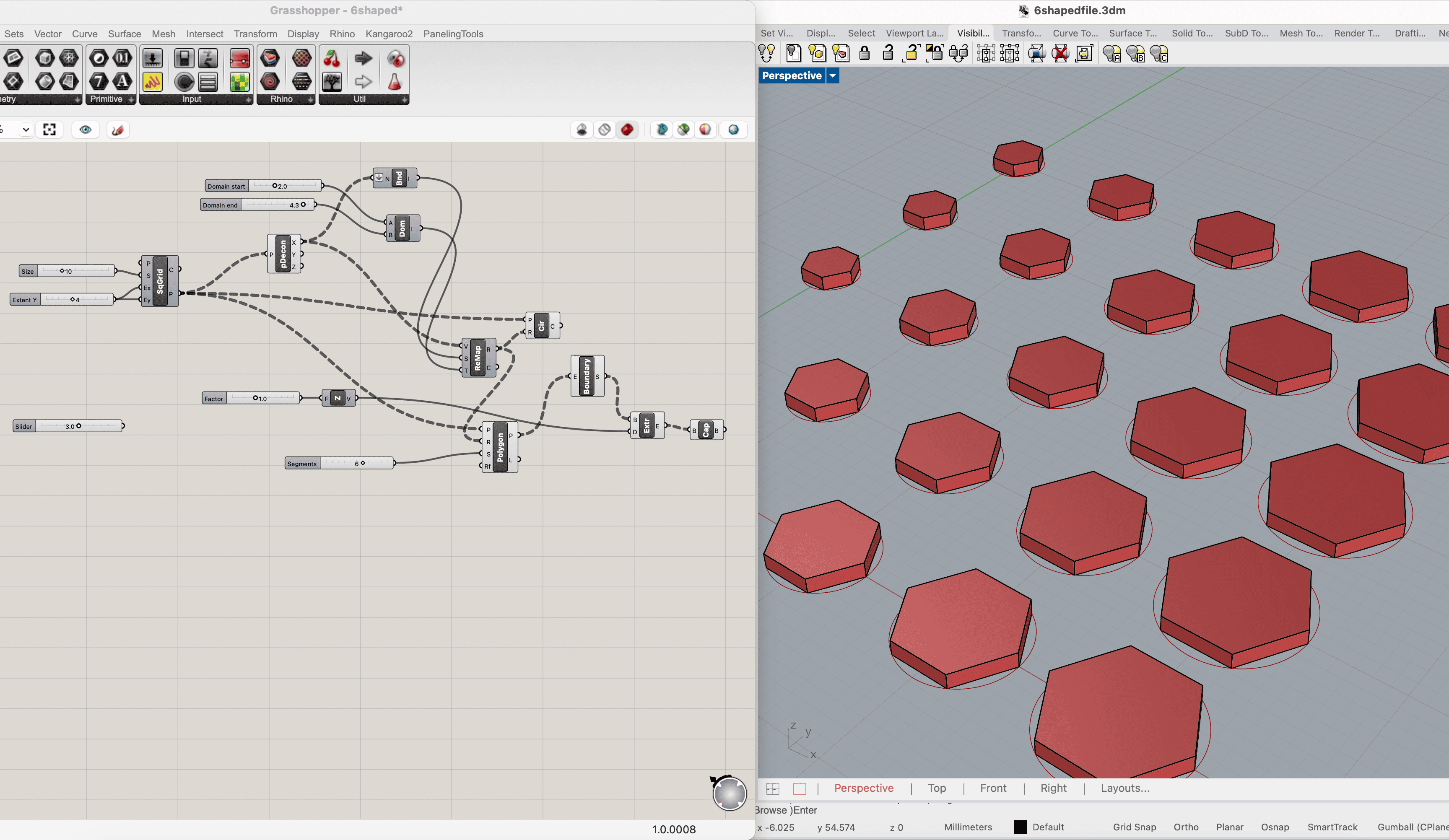
For my first experiment, I created a grid of hexagonal elements that gradually change in size across the pattern. I then added thickness to turn the flat shapes into three-dimensional elements.
Understanding the Grasshopper Interface
Grasshopper works by connecting components rather than drawing every shape manually.
- Component: A box that performs an operation, such as creating a grid or extruding a surface.
- Input: A connection point on the left side of a component, where information enters.
- Output: A connection point on the right side, where the result leaves.
- Wire: A connection that transfers information between components.
- Number Slider: An adjustable number used to control a parameter, such as spacing, radius, or thickness.
To add a component, I double-clicked an empty area of the Grasshopper canvas, typed its name, and selected it from the search results.
To connect two components, I dragged a wire from the output of the first component to the input of the next.
1. Opening Rhino and Grasshopper
- I opened a new Rhino document using millimeters as the model units.
- I typed
Grasshopperinto the Rhino command line and pressed Enter. - This opened the Grasshopper window, where I built the connections that generated my pattern.
- I arranged Rhino and Grasshopper side by side so I could see the geometry update while changing the definition.
The geometry generated in Grasshopper appeared as a preview in the Rhino viewport.
2. Creating a Grid of Points
The first step was to create evenly spaced positions for the repeated shapes.
- I double-clicked the Grasshopper canvas.
- Searched for Square Grid and placed the component.
- I added a Number Slider by double-clicking the canvas, typing
10, and pressing Enter. - I connected this slider to the grid’s S - Size input.
This value controlled the grid spacing. With the Rhino document set to millimeters, a value of 10 created a spacing of 10 mm between neighboring grid points.
- I added another slider with a value of
4. - I connected it to Ey - Extent Y, which controlled the number of grid cells in the Y direction.
The Ex - Extent X input controlled the number of cells in the other direction. To make this value adjustable as well, a separate whole-number slider can be connected to Ex.
The Square Grid component produced two outputs:
- C - Cells: The square grid outlines.
- P - Points: The grid points used to position the repeated shapes.
For the next steps, I used the P output.
3. Extracting the Position of Each Point
I wanted the shapes to change size according to their position across the grid.
Each point has three coordinates:
- X: Position along the X axis.
- Y: Position along the Y axis.
-
Z: Position along the Z axis.
-
I added a Deconstruct Point component.
- Connected the Square Grid’s P output to Deconstruct Point’s P input.
- This separated each point into its X, Y, and Z values.
- I used the X output to control the size variation.
Because I used X, points with the same X coordinate received the same size value. The sizes changed as the points progressed along the X direction.
4. Finding the Existing Range of Values
The X coordinates described the positions of the points, but I needed to convert them into suitable sizes for my shapes.
- I added a Bounds component.
- I connected the X output of Deconstruct Point to the N input of Bounds.
Bounds found the smallest and largest values in the connected data. These limits defined the starting range for the size calculation.
For example, position values might range from 0 to 40, while the desired shape radii might range from 2 to 4.3 mm. Remapping converts the first range into the second.
5. Setting the Minimum and Maximum Shape Sizes
Next, I defined the size range I wanted to use.
- I added a Construct Domain component.
- I created two Number Sliders:
- Domain start:
2.0 - Domain end:
4.3 - I connected the 2.0 slider to A.
- I connected the 4.3 slider to B.
A domain is an interval between two numbers. In this case, the domain defined the target radius range from 2.0 to 4.3 mm.
These values controlled the polygon’s radius, measured from its center to a corner. They did not represent its full width.
6. Remapping Positions into Shape Sizes
I used Remap Numbers to translate the point positions into the chosen radius range.
- I added a Remap Numbers component.
- I connected the X output from Deconstruct Point to V - Values.
- I connected the output of Bounds to S - Source domain.
- I connected the output of Construct Domain to T - Target domain.
The inputs performed the following roles:
| Input | Purpose |
|---|---|
| V - Values | The X coordinates to convert |
| S - Source domain | The original range of those coordinates |
| T - Target domain | The desired radius range: 2.0-4.3 mm |
The R output provided the new radius values. Smaller X values produced smaller radii, while larger X values produced larger radii.
7. Creating the Hexagonal Pattern
Once the positions and radius values were ready, I created the repeated shapes.
- I added a Polygon component.
- I connected the Square Grid’s P output to the Polygon’s P — Plane input.
Grasshopper used the points to position the polygons on planes parallel to the XY plane.
- I connected the R output of Remap Numbers to the Polygon’s R — Radius input.
- I created a whole-number slider with a value of
6. - I connected it to S — Segments.
The segment count determined the number of sides. A value of six created hexagons.
At this stage, the pattern consisted of closed, flat polygon outlines. The shapes had positions and sizes, but no surfaces or thickness.
8. Turning the Outlines into Surfaces
To fill the hexagonal outlines, I created planar surfaces.
- I added a Boundary Surfaces component.
- I connected the Polygon’s P output to Boundary Surfaces’ E — Edges input.
Boundary Surfaces created a flat surface inside each closed hexagon.
The curves needed to be closed and planar for this operation to work correctly.
9. Defining the Extrusion Direction and Thickness
To give the surfaces thickness, I needed to specify both a direction and a distance.
- I added a Unit Z component.
- I created a Number Slider with a value of
1.0. - I connected it to Unit Z’s F — Factor input.
Unit Z created a vector pointing along the positive Z axis, perpendicular to the XY grid.
The factor controlled the vector’s length. With millimeter units, a value of 1.0 produced an extrusion distance of 1 mm.
10. Extruding the Surfaces
- I added an Extrude component.
- I connected the S output of Boundary Surfaces to Extrude’s B — Base input.
- I connected the V output of Unit Z to Extrude’s D — Direction input.
This extended each flat hexagonal surface upward by the specified distance.
Changing the slider connected to Unit Z changed the thickness of all the elements together.
11. Capping the Extrusions
- I added a Cap Holes component.
- I connected Extrude’s E output to Cap Holes’ B input.
Cap Holes closes planar openings in the extruded geometry. This was the final component in my definition.
Before exporting for printing, I still needed to check that the resulting objects were valid and closed.
12. Viewing the Result Clearly
To inspect the three-dimensional shapes, I changed the Rhino viewport to Shaded using the menu beside the viewport name.
Grasshopper can preview several stages of a definition at the same time. This can leave construction curves visible around the final objects.
To display only the final result:
- I selected the earlier geometry-producing components, such as Square Grid, Circle, Polygon, Boundary Surfaces, and Extrude.
- I right-clicked and turned their Preview off.
- I kept the preview of Cap Holes on.
Turning Preview off only hides that component’s geometry. It does not interrupt its connections or stop the definition from working.
Adjustable Parameters
My definition allowed me to explore the pattern through the following controls:
| Parameter | What it changes |
|---|---|
| Grid size | Spacing between neighboring grid points |
| Grid extents | Number of grid cells in each direction |
| Domain start | Smallest polygon radius |
| Domain end | Largest polygon radius |
| Polygon segments | Number of sides of each polygon |
| Unit Z factor | Extrusion thickness |
Changing these values updated the connected geometry automatically, allowing me to test variations without rebuilding the pattern.
Initial Result
The result was a grid of separate hexagonal elements with gradually changing sizes and a consistent thickness. the elements were not connected to each other as it will be printed on fabric.
Exploring Pattern Variations
After building the initial definition, I experimented with its parameters to understand how each one affected the pattern. The connected setup allowed me to make changes and immediately observe the result in Rhino.
Changing the Element Sizes
I adjusted the two sliders connected to Construct Domain to change the range of element sizes.
Bringing the minimum and maximum values closer together produced a more uniform pattern. Increasing the difference between them made the size gradient more noticeable.
The values controlled the radius of each element, rather than its full width.
Changing the Shape
I initially explored circles before replacing them with polygons. Using the Polygon component allowed me to control the number of sides through the Segments input.
For the hexagonal version, I set the segment count to six. This changed the outline while keeping the grid positions and size-control system.
Adjusting the Spacing
The Size input of Square Grid controlled the distance between neighboring grid points. Changing this value affected the gaps between the elements.
Adding Thickness
I used the slider connected to Unit Z to control the extrusion thickness. This allowed me to give all the elements the same height while keeping their different sizes.
Parameters of the Initial Hexagonal Sample
| Parameter | Value |
|---|---|
| Rhino model units | Millimeters |
| Grid spacing | 10 mm |
| Grid extent Y | 4 cells |
| Minimum polygon radius | 2.0 mm |
| Maximum polygon radius | 4.3 mm |
| Polygon sides | 6 |
| Extrusion thickness | 1.0 mm |
3. Tools
Results & documentation
- Don’t forget to document the outcome including:
- Upload the photos & files on oscircularfashion
- Final result
- Photos from different stages
- Videos of movement or interaction, show how a material moves, something was assembled or the interactive
- Include measurements or a reference object to give a sense of size
- Describe the (material) properties or what you made
- Comparison between attempts, if you did multiple experiments or generated multiple files before fabricating / deploying. You can use a table as shown in week 4
Weekly reflection & critical thinking
- What did I learn? What did I personally find interesting or surprised me?
- What would I do differently? If something "failed" do I know how else to tackle it now?"
- How does this connect to my final project or my learning trajectory?
- What are implications and possible applications, think also from the ethical or environmental aspect, how it could connect to your practice and project?
Fabrication files & References
-
File: Grasshopper definition.. ↩
-
Reference: Author; Title; Source; year ↩